
Bugs Exist In All Code Bases
One of the most common misconceptions among new programmers is that experienced developers write bug-free code. Spend enough time programming, however, and you'll discover an important truth:
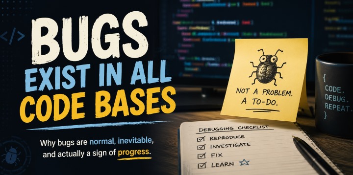
Bugs exist in all code bases.
It doesn't matter if the project is a weekend hobby, an indie game, a commercial application, or software used by millions of people. Given enough complexity, enough features, and enough time, bugs will find their way into the code.
Perfection Is an Impossible Target
Programming isn't simply writing instructions for a computer. It's about solving problems, and those problems often change over time. New features are added, old systems are updated, and user expectations evolve.
Every change introduces the possibility of unintended side effects.
A fix for one problem might expose another. An optimisation could create an edge case that nobody anticipated. A new feature might interact with older code in unexpected ways.
This isn't necessarily bad programming. It's simply the nature of software development.
Complexity Is the Real Enemy
A program might start out as a few hundred lines of code. Years later, it could have hundreds of thousands of lines spread across countless functions and modules.
The more moving parts a project has, the more interactions exist between those parts.
Even if each individual function works perfectly, combining them can produce behaviours that weren't expected.
The challenge isn't eliminating every possible bug. It's managing complexity so that bugs are easier to find and fix.
Every Programmer Writes Bugs
Beginners often think they're making mistakes because they aren't good enough.
Professionals know that mistakes are part of the job.
Experienced programmers don't magically avoid bugs. They simply develop better habits:
* Breaking problems into smaller pieces.
* Testing code frequently.
* Writing clear, readable functions.
* Using debugging tools effectively.
* Accepting that the first version probably won't be the final version.
The difference between a beginner and an experienced developer isn't the number of bugs they create.
It's how quickly they can track them down and fix them.
Finding Bugs Is Progress
It's easy to become frustrated when a bug appears after hours of coding.
In reality, discovering a bug is often a success.
You found something that wasn't working correctly before your users did. You learned something about your program. You made the code a little more robust than it was yesterday.
Every bug fixed improves the quality of the project.
Even Famous Software Has Bugs
* Operating systems have bugs.

* Games have bugs.

* Web browsers have bugs.

* Programming languages have bugs.
The tools we use every day receive updates and patches because developers continually discover issues and improve their software.
If some of the largest software projects in the world can't eliminate every bug, it's unrealistic to expect our own projects to be perfect.
The Goal Is Better Software
Good software development isn't about creating bug-free code.
It's about creating code that can be understood, maintained, tested, and improved over time.
A healthy code base isn't one without bugs.
It's one where bugs can be identified, fixed, and prevented from causing bigger problems in the future.
Final Thoughts
Bugs exist in all code bases.
That's not a sign that a project has failed or that a programmer lacks skill. It's a natural consequence of building increasingly complex systems to solve increasingly complex problems.
The next time you encounter a bug, remember that you're participating in a process shared by every programmer, from hobbyists writing their first game to engineers maintaining software used around the world.
The goal isn't perfection.
The goal is to make today's code a little better than yesterday's.


